The Grammar of Graphics
Meet the Palmer Penguins ![]()

# A tibble: 344 × 8
   species island    bill_length_mm bill_depth_mm flipper_length_mm body_mass_g
   <fct>   <fct>              <dbl>         <dbl>             <int>       <int>
 1 Adelie  Torgersen           39.1          18.7               181        3750
 2 Adelie  Torgersen           39.5          17.4               186        3800
 3 Adelie  Torgersen           40.3          18                 195        3250
 4 Adelie  Torgersen           NA            NA                  NA          NA
 5 Adelie  Torgersen           36.7          19.3               193        3450
 6 Adelie  Torgersen           39.3          20.6               190        3650
 7 Adelie  Torgersen           38.9          17.8               181        3625
 8 Adelie  Torgersen           39.2          19.6               195        4675
 9 Adelie  Torgersen           34.1          18.1               193        3475
10 Adelie  Torgersen           42            20.2               190        4250
# ℹ 334 more rows
# ℹ 2 more variables: sex <fct>, year <int>Question: In terms of the way they are constructed…
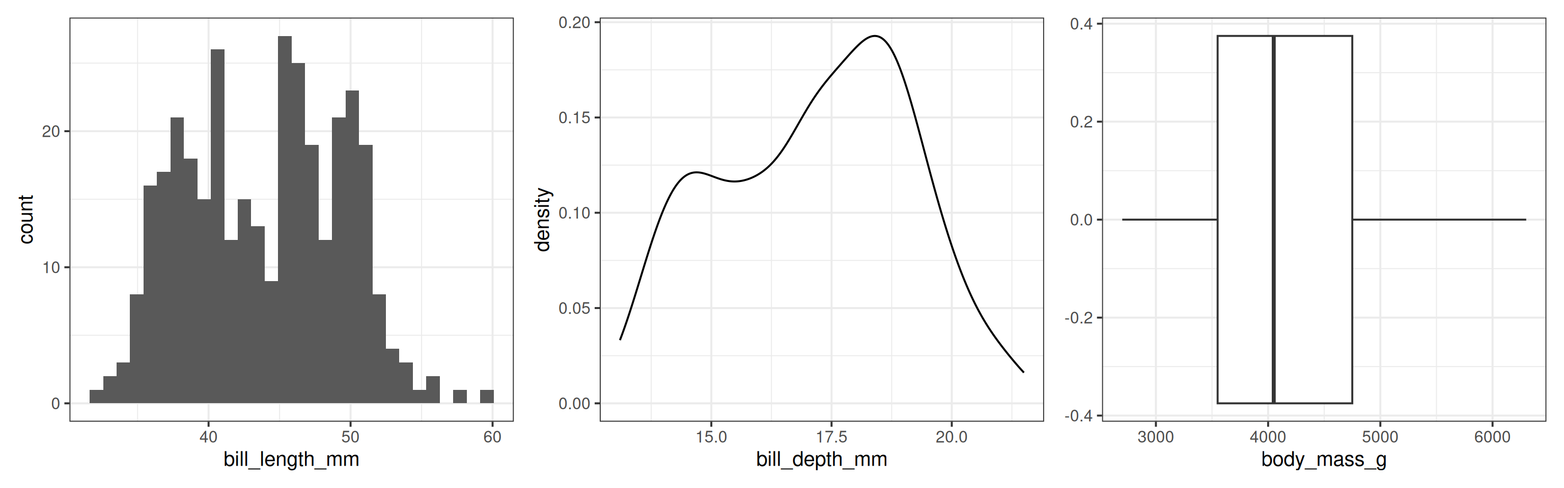
What do these plots have in common? How do they differ?
01:20
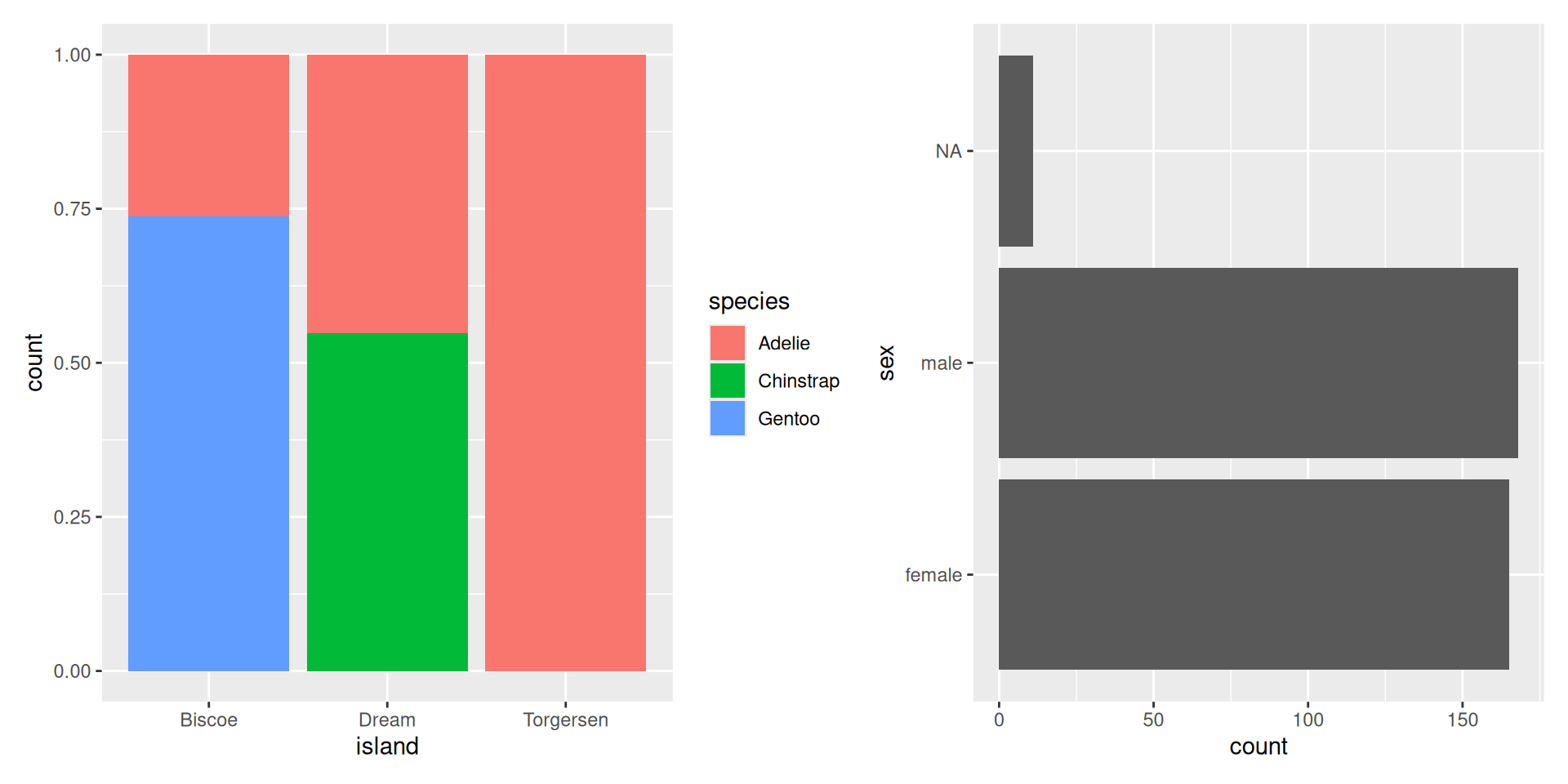
Question: What do these plots have in common? How do they differ?
01:20
“The Grammar of Graphics”
Leland Wilkinson (1999)
- A grammar to describes all statistical graphics.
- Underlies most modern data visualization software.

Aesthetic Mapping
An aesthetic mapping links a variable in the data to a visual channel that can encode its variation.
Channels for ordered variables

Aesthetic Mapping
An aesthetic mapping links a variable in the data to a visual channel that can encode its variation.
Channels for unordered variables

Redux 1

Redux 1

Question: What are the aesthetic mappings and geometries used here?

01:30


# A tibble: 344 × 3
   bill_length_mm flipper_length_mm species
            <dbl>             <int> <fct>
 1           39.1               181 Adelie
 2           39.5               186 Adelie
 3           40.3               195 Adelie
 4           NA                  NA Adelie
 5           36.7               193 Adelie
 6           39.3               190 Adelie
 7           38.9               181 Adelie
 8           39.2               195 Adelie
 9           34.1               193 Adelie
10           42                 190 Adelie
# ℹ 334 more rows
