US Presidential Elections 2020
Mapping Elections Data I
Required Packages
The content in these slides depend on the following packages:
About
Visualizing US Presidential Elections (2020)
US Presidential Elections 2020
Data from MIT Election Lab

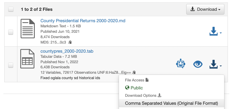
County Presidential Election (2000-2020)

https://dataverse.harvard.edu/dataset.xhtml?persistentId=doi:10.7910/DVN/VOQCHQ
Citation: Data Source
Data: County Presidential Election Returns 2000-2020
Source: MIT Election Data + Science Lab
https://dataverse.harvard.edu/dataset.xhtml?persistentId=doi:10.7910/DVN/VOQCHQ
MIT Election Data and Science Lab, 2018, “County Presidential Election Returns 2000-2020”, https://doi.org/10.7910/DVN/VOQCHQ, Harvard Dataverse, V11, UNF:6:HaZ8GWG8D2abLleXN3uEig== [fileUNF]
License: Public Domain CC0 1.0
Data Available in CSV format
US Presidential Election 2000-2020 Data
CSV file available in bCourses (see Files/data)
US Presidential Election 2000-2020 Data
# A tibble: 8 × 6
   year state   state_po county_name county_fips office
  <int> <chr>   <chr>    <chr>       <chr>       <chr>
1  2000 alabama AL       autauga     01001       US PRESIDENT
2  2000 alabama AL       autauga     01001       US PRESIDENT
3  2000 alabama AL       autauga     01001       US PRESIDENT
4  2000 alabama AL       autauga     01001       US PRESIDENT
5  2000 alabama AL       baldwin     01003       US PRESIDENT
6  2000 alabama AL       baldwin     01003       US PRESIDENT
7  2000 alabama AL       baldwin     01003       US PRESIDENT
8  2000 alabama AL       baldwin     01003       US PRESIDENT
US Presidential Election 2000-2020 Data (cont’d)
# A tibble: 10 × 6
   candidate      party      candidatevotes totalvotes  version mode
   <chr>          <chr>               <dbl>      <dbl>    <dbl> <chr>
 1 AL GORE        DEMOCRAT             4942      17208 20220315 TOTAL
 2 GEORGE W. BUSH REPUBLICAN          11993      17208 20220315 TOTAL
 3 RALPH NADER    GREEN                 160      17208 20220315 TOTAL
 4 OTHER          OTHER                 113      17208 20220315 TOTAL
 5 AL GORE        DEMOCRAT            13997      56480 20220315 TOTAL
 6 GEORGE W. BUSH REPUBLICAN          40872      56480 20220315 TOTAL
 7 RALPH NADER    GREEN                1033      56480 20220315 TOTAL
 8 OTHER          OTHER                 578      56480 20220315 TOTAL
 9 AL GORE        DEMOCRAT             5188      10395 20220315 TOTAL
10 GEORGE W. BUSH REPUBLICAN           5096      10395 20220315 TOTAL
2020 Presidential Election
Let’s focus on the 2020 Presidential Election
2020 Presidential Election, California Results
dat2020 |>
  filter(state == "california") |>
  select(county_name, candidate:totalvotes) |>
  slice_head(n = 5)
# A tibble: 5 × 5
county_name candidate party candidatevotes totalvotes
<chr> <chr> <chr> <dbl> <dbl>
1 alameda JOSEPH R BIDEN JR DEMOCRAT 617659 770070
2 alameda OTHER GREEN 4664 770070
3 alameda JO JORGENSEN LIBERTARIAN 6295 770070
4 alameda OTHER OTHER 5143 770070
5 alameda DONALD J TRUMP REPUBLICAN 136309 770070Expressing votes relative to total in county
Let’s add a column propvotes to get the proportion of votes that each candidate obtained in every county:
propvotes = candidatevotes / totalvotes
Analysis of California
Number of votes that each candidate received in each of the counties in California
# A tibble: 232 × 3
# Groups:   county_name [58]
   county_name candidate         sum_votes
   <chr>       <chr>                 <dbl>
 1 alameda     DONALD J TRUMP       136309
 2 alameda     JO JORGENSEN           6295
 3 alameda     JOSEPH R BIDEN JR    617659
 4 alameda     OTHER                  9807
 5 alpine      DONALD J TRUMP          244
 6 alpine      JO JORGENSEN             15
 7 alpine      JOSEPH R BIDEN JR       476
 8 alpine      OTHER                     6
 9 amador      DONALD J TRUMP        13585
10 amador      JO JORGENSEN            349
# ℹ 222 more rows
Maps
Map of US (contiguous states)
We’ve seen how to plot a map of US
Map of US (contiguous states)

Map of US Counties
"rnaturalearth" does not come with a built-in map data of US Counties. But we can use the "county" map-data from the package "maps".
To be consistent with the way we handle vector data, we convert the "county" map object into an "sf" object with st_as_sf().
Map of US Counties

Map of California Counties
Map Data of California Counties
We have map-data of US states:
us_states_sfWe have map-data of US counties:
us_counties_sfIt would be nice to have map-data of California Counties.
How do get map-data of California Counties? This requires a bit of string matching via str_detect():
Map of California Counties
With filtered counties of California cal_counties_sf, we can make a map:
Map of California Counties

What’s in cal_counties_sf?
Simple feature collection with 10 features and 1 field
Geometry type: MULTIPOLYGON
Dimension:     XY
Bounding box:  xmin: -124.2344 ymin: 35.90154 xmax: -118.3502 ymax: 42.00927
Geodetic CRS:  +proj=longlat +ellps=clrk66 +no_defs +type=crs
                        ID                           geom
1       california,alameda MULTIPOLYGON (((-121.4785 3...
2        california,alpine MULTIPOLYGON (((-120.0748 3...
3        california,amador MULTIPOLYGON (((-120.0748 3...
4         california,butte MULTIPOLYGON (((-121.6217 3...
5     california,calaveras MULTIPOLYGON (((-120.069 38...
6        california,colusa MULTIPOLYGON (((-121.8223 3...
7  california,contra costa MULTIPOLYGON (((-121.5702 3...
8     california,del norte MULTIPOLYGON (((-123.6844 4...
9     california,el dorado MULTIPOLYGON (((-121.1519 3...
10       california,fresno MULTIPOLYGON (((-120.6821 3...
Adding Column of County Name
For sake of convenience, we need to add a column county to the map-data cal_counties_sf (so that we have the name of the county)
cal_counties_sf = cal_counties_sf |>
  mutate(county = str_remove(ID, "california,"))

head(cal_counties_sf$county)
[1] "alameda" "alpine" "amador" "butte" "calaveras" "colusa" What relevant data do we have so far?
2020 votes-data from California:
votes_californiaMap-data of California counties:
cal_counties_sf
We need to join these data sets in order to combine the votes information with the map-data.
Joining map-data with elections-data
Join California map-data with votes-data, via inner_join()
Joining map-data with elections-data
Simple feature collection with 8 features and 5 fields
Geometry type: MULTIPOLYGON
Dimension:     XY
Bounding box:  xmin: -122.2749 ymin: 37.45998 xmax: -119.5362 ymax: 38.90956
Geodetic CRS:  +proj=longlat +ellps=clrk66 +no_defs +type=crs
                  ID  county         candidate propvotes candidatevotes
1 california,alameda alameda JOSEPH R BIDEN JR      0.80         617659
2 california,alameda alameda             OTHER      0.01           4664
3 california,alameda alameda      JO JORGENSEN      0.01           6295
4 california,alameda alameda             OTHER      0.01           5143
5 california,alameda alameda    DONALD J TRUMP      0.18         136309
6  california,alpine  alpine JOSEPH R BIDEN JR      0.64            476
7  california,alpine  alpine             OTHER      0.01              4
8  california,alpine  alpine      JO JORGENSEN      0.02             15
                            geom
1 MULTIPOLYGON (((-121.4785 3...
2 MULTIPOLYGON (((-121.4785 3...
3 MULTIPOLYGON (((-121.4785 3...
4 MULTIPOLYGON (((-121.4785 3...
5 MULTIPOLYGON (((-121.4785 3...
6 MULTIPOLYGON (((-120.0748 3...
7 MULTIPOLYGON (((-120.0748 3...
8 MULTIPOLYGON (((-120.0748 3...
Mapping Votes (facet by candidate)

Looking for an alternative color scheme
We can use a Viridis Color palette.
https://ggplot2.tidyverse.org/reference/scale_viridis.html
The function scale_fill_viridis_c() allows us to choose a continuous scale.
Its argument direction = -1 gives a reversing order (from yellow to dark blue).
Mapping Votes (5th attempt)

Map of Joe Biden’s votes

Joe Biden’s votes: top-5 counties
votes_california |>
  filter(candidate == "JOSEPH R BIDEN JR") |>
  arrange(desc(propvotes)) |>
  slice_head(n = 5)
# A tibble: 5 × 4
county_name candidate propvotes candidatevotes
<chr> <chr> <dbl> <dbl>
1 san francisco JOSEPH R BIDEN JR 0.85 378156
2 marin JOSEPH R BIDEN JR 0.82 128288
3 alameda JOSEPH R BIDEN JR 0.8 617659
4 santa cruz JOSEPH R BIDEN JR 0.79 114246
5 san mateo JOSEPH R BIDEN JR 0.78 291496Joe Biden’s votes: bottom-5 counties
votes_california |>
  filter(candidate == "JOSEPH R BIDEN JR") |>
  arrange(propvotes) |>
  slice_head(n = 5)
# A tibble: 5 × 4
county_name candidate propvotes candidatevotes
<chr> <chr> <dbl> <dbl>
1 lassen JOSEPH R BIDEN JR 0.23 2799
2 modoc JOSEPH R BIDEN JR 0.26 1150
3 tehama JOSEPH R BIDEN JR 0.31 8911
4 shasta JOSEPH R BIDEN JR 0.32 30000
5 glenn JOSEPH R BIDEN JR 0.35 3995Map with ggplotly()
View code
joe_biden = cal_votes_map |>
  filter(candidate == "JOSEPH R BIDEN JR")

joe_biden_map = ggplot(data = joe_biden, aes(label = county)) +
  geom_sf(aes(fill = propvotes)) +
  scale_fill_viridis_c(name = "Prop. of Votes", direction = -1) +
  theme_void() +
  labs(title = "Joe Biden's Proportion of Votes")

ggplotly(joe_biden_map)